Splitting structure data using Union-Find
Curating and organizing good training, testing and validation datasets is a vital component of effective machine learning pipelines. Machine learning models are extemely good at ferreting out statistical regularities in your data, leading to unrealistic indicators of model performance. Ensuring that your training and testing splits are reflective of the differences in data distribution your model will encounter in actual usage helps to identify issues early on.
This is especially important when our datasets do not conform to the independent and identically distributed (i.i.d) assumption, i.e. when there is an inherant ‘grouping’ or dependance between rows in our dataset. This assumption is often violated when we train models on protein structure datasets, as protein complexes are composed of subunits that may be shared across multiple complexes. Building training sets with these datasets therefore requires more care. In this post I will be exploring the Union-Find (UF) algorithm as a method to ensure correct stratification of protein complexes into train and test splits for modelling.
Why is splitting protein structure data tricky?
Proteins are often composed of multimeric complexes - that is multiple polypeptide chains that associate with one another. The individual polypeptide chains in a protein complex are termed subunits, and these subunits (or closely related family groupings of a subunit) can associate with multiple different partners. This composable nature of proteins is part of what makes them so powerful, as a smaller number of ‘functions’ can mix-and-match to create a much larger repertoire of behaviours. The PDB database is an amazing online resource that compiles 3D models of these protein complexes, and it is this dataset that was used to develop the AlphaFold family of models, as well as numerous other protein folding models. In addition to its use in powering folding models, increasingly this dataset is being used as input to systems that predict properties of proteins, such as their biophysical behaviour or function.
In order to prepare a dataset from this resource for model training, one might naïvely take some fraction of protein structures and put them in training, validation and testing sets. Unfortunately, this will likely lead to the unrealistic performance indicators discussed in the opening paragraph, Why? Because some protein structures will share a high degree of similarity with one other proteins in the dataset. Models perform better on data that is very similar to that which it has seen in its training set (where it has been shown the labels), and so testing on these examples will mean the model appears to be performing very well. This is a problem, as often we will want to use our model on novel proteins that are further from our training samples. Knowing how our model performs on these novel proteins is essential if we want to be confident in using our model.
One approach is to cluster proteins by their similarity (often sequence similarity), and then pick out a representative member from each cluster as a training example. This turns out to be tricky, due to the modular nature of protein complexes discussed previously. The following example demonstrates why. Imagine we have 3 protein complexes composed of 4 subunits: A-B, B-C, C-D (shown in image). No two complexes are the same, but each shares a subunit with one other complex. If we place A-B and B-C in the training set, then the model will be able to use the information we gave it for B-C directly on C-D, as the C subunit is shared. If we instead put A-B and C-D in the training set and B-C in the test set, then the model would be able to use the information from the B subunit as it is shared with B-C. It turns out that there is no way to split these complexes into testing and training datasets that doesn’t ‘leak’ information from the training set via shared subunits.
import networkx as nx
import matplotlib.pyplot as plt
G = nx.DiGraph()
G.add_edges_from([('A', 'B'), ('B', 'C'), ('C', 'D')])
pos = {'A': (0, 1), 'B': (1, 1), 'C': (1, 0), 'D': (0, 0)}
nx.draw_networkx_nodes(G, pos, node_color='skyblue', node_size=1000)
nx.draw_networkx_edges(G, pos, edgelist=[('A', 'B')], edge_color='green', width=2, arrowsize=20)
nx.draw_networkx_edges(G, pos, edgelist=[('B', 'C')], edge_color='blue', width=2, arrowsize=20)
nx.draw_networkx_edges(G, pos, edgelist=[('C', 'D')], edge_color='red', width=2, arrowsize=20)
nx.draw_networkx_labels(G, pos, font_weight='bold')
plt.title("Box-Shaped Path Graph")
plt.axis('off')
plt.show()
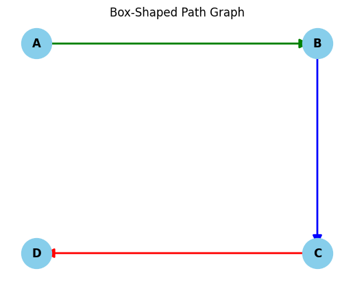
We can view our protein comples dataset as disjoint subgraphs, where each instance like the one in the image above represents a connected component in our graph. We must ensure that each connected component in our dataset ends up in either our training set or our test set, but does not straddle both. Of course, the connected components are not given to us, we have to find them. This is where the UF algorithm comes in handy, but first we will need a dataset, and a method of clustering the protein sequences in the dataset to create the input for the UF algorithm.
The dataset
The dataset we will use is the SabDab dataset hosted by the Oxford Protein Informatics Group (OPIG). You can find it here. This dataset contains a subset of the PDB with structures that are either antibodies, or antibodies bound to their ligands. There are a few steps we need to do in order to prepare the data to be used as input the the UF algorithm. We need to:
- Filter only antibodies that are complexed with protein antigens
- Select a representative from the complexes in each file (PDB files will often contain multiple copies of the complex)
- Convert each PDB file to a FASTA file so it can be clustered by a sequence clustering algorithm
- Pool the FASTA files into one big fasta file, retaining the identity of the original PDB file each record came from
- Cluster to sequences in the FASTA file
Lets start by filtering antibody complexes that have protein antigens.
$ls ~/datasets/all_structures/imgt/* | xargs grep -PH 'AGTYPE=PROTEIN(;PROTEIN)*$'  | head
# output
~/datasets/all_structures/imgt/1a14.pdb:REMARK   5 PAIRED_HL HCHAIN=H LCHAIN=L AGCHAIN=N AGTYPE=PROTEIN
~/datasets/all_structures/imgt/1a2y.pdb:REMARK   5 PAIRED_HL HCHAIN=B LCHAIN=A AGCHAIN=C AGTYPE=PROTEIN
~/datasets/all_structures/imgt/1adq.pdb:REMARK   5 PAIRED_HL HCHAIN=H LCHAIN=L AGCHAIN=A AGTYPE=PROTEIN
~/datasets/all_structures/imgt/1afv.pdb:REMARK   5 PAIRED_HL HCHAIN=H LCHAIN=L AGCHAIN=A AGTYPE=PROTEIN
~/datasets/all_structures/imgt/1afv.pdb:REMARK   5 PAIRED_HL HCHAIN=K LCHAIN=M AGCHAIN=B AGTYPE=PROTEIN
...
This pulls out the REMARK metadata lines from files with protein only antigens. As you can see some files contain multiple copies of the antibody-antigen chains. This is just an artifact of the way that crystallography is done. We only need one copy of each for our dataset so we will (somewhat arbitrarily) pick the first one from each file. We could select one based on the best resolution, but I will leave that as an excercise for the reader. We can remove the duplicates and clean up the line a bit with the command below.
$ls ~/datasets/all_structures/imgt/* |
    xargs grep -PH 'AGTYPE=PROTEIN(;PROTEIN)*$' |
    awk '!seen[$1]++' |                                                                          # drop dupicates
    sed -E -e 's/:REMARK   5 [^ ]+/' -e 's/AGTYPE=PROTEIN.*$//g' -e 's/[^ ]+=//g' -e 's/ $//' | # clean up the line
    awk 'NF==4 {print $0}; NF==3 {print $1,$2,"-",$3}' |                                         # insert a placeholder for the light chain column in single chain antibodies
    sed '1i\path H L Ag' |                                                                       # insert a header
    tr ' ' $'\t' |                                                                               # convert it to csv
    tee lookup.tsv                                                                               # create a lookup.csv file and print the output
# output
~/datasets/all_structures/imgt/1a14.pdb H L N
~/datasets/all_structures/imgt/1a2y.pdb B A C
~/datasets/all_structures/imgt/1adq.pdb H L A
~/datasets/all_structures/imgt/1afv.pdb H L A
...
Ok, we now have the set of files that will ultimately form our dataset. We next have to convert these files to fasta files and pool them together so they can be clustered. Mungeing PDB files can get hairy, but luckily the fantastic pdb-tools exists, which can do alot of this for us. This is some heavy duty text processing we are doing here so we will want to do it in parallel. My favourite tool for doing parallel processing is GNU parallel (maybe my favourite tool full stop!) so I will use that, although xargs is also a good option. We will select just the antigen chains to cluster for this post.
$mkdir -p fastas && cut -f1,4 lookup.tsv |  # select the antigen chain IDs
    sed 's/;/,/g' |                         # change the antigen chain separator to be compatible with the arguments to pdb-tools
    sed 1d |                               # remove the header
    parallel --eta --colsep=$'\t' 'pdb_selchain -{2} {1} | pdb_delhetatm | pdb_tofasta -multi > fastas/{1/.}.fasta' # select the antigen chains, remove hetatms then convert them to fastas
The result of this will be a folder with a set of fastas that look like this.
$cat fastas/1a14.fasta
>PDB|N
RDFNNLTKGLCTINSWHIYGKDNAVRIGEDSDVLVTREPYVSCDPDECRFYALSQGTTIR
GKHSNGTIHDRSQYRALISWPLSSPPTVYNSRVECIGWSSTSCHDGKTRMSICISGPNNN
ASAVIWYNRRPVTEINTWARNILRTQESECVCHNGVCPVVFTDGSATGPAETRIYYFKEG
KILKWEPLAGTAKHIEECSCYGERAEITCTCRDNWQGSNRPVIRIDPVAMTHTSQYICSP
VLTDNPRPNDPTVGKCNDPYPGNNNNGVKGFSYLDGVNTWLGRTISIASRSGYEMLKVPN
ALTDDKSKPTQGQTIVLNTDWSGYSGSFMDYWAEGECYRACFYVELIRGRPKEDKVWWTS
NSIVSMCSSTEFLGQWDWPDGAKIEYFL
CD-Hit takes a single fasta file so we need to combine these, but as you can see, there is no identifying information in the fasta file that can be used to identify which sequences came from which file once they have been pooled. We can rectify this with awk by inserting the filename in the place of the “PDB” string in the ID field.
awk '/>PDB/ {sub("PDB", FILENAME)}; {print}' fastas/* > seqs.fasta
#output
...
>fastas/9uxd.fasta|A
QCVNLTTRTQLPPAYTNSFTRGVYYPDKVFRSSVLHSTQDLFLPFFSNVTWFHAIHKRFD
NPVLPFNDGVYFASTEKSNIIRGWIFGTTLDSKTQSLLIVNNATNVVIKVCEFQFCNDPF
LGVYYHKNNKSWMESEFRVYSSANNCTFEYVSQPFLMDLEGKFKNLREFVFKNIDGYFKI
YSKHTPINLVRDLPQGFSALEPLVDLPIGINITRFQTLLALHRSYLTPGDSSSGWTAGAA
AYYVGYLQPRTFLLKYNENGTITDAVDCALDPLSETKCTLKSFTVEKGIYQTSNFRVQPT
ESIVRFPNITNLCPFGEVFNATRFASVYAWNRKRISNCVADYSVLYNSASFSTFKCYGVS
PTKLNDLCFTNVYADSFVIRGDEVRQIAPGQTGKIADYNYKLPDDFTGCVIAWNSNNLDS
KVGGNYNYLYRLFRKSNLKPFERDISTEIYQAGSTPCNGVEGFNCYFPLQSYGFQPTNGV
GYQPYRVVVLSFELLHAPATVCGPKKSTNLVKNKCVNFNFNGLTGTGVLTESNKKFLPFQ
QFGRDIADTTDAVRDPQTLEILDITPCSFGGVSVITPGTNTSNQVAVLYQDVNCTEVPNV
FQTRAGCLIGAEHVNNSYECDIPIGAGICASYQQSIIAYTMSLGAENSVAYSNNSIAIPT
NFTISVTTEILPVSMTKTSVDCTMYICGDSTECSNLLLQYGSFCTQLNRALTGIAVEQDK
NTQEVFAQVKQIYKTPPIKDFGGFNFSQILPDPSKPSKRSPIEDLLFNKVTLFNGLTVLP
PLLTDEMIAQYTSALLAGTITSGWTFGAGPALQIPFPMQMAYRFNGIGVTQNVLYENQKL
IANQFNSAIGKIQDSLSSTPSALGKLQDVVNQNAQALNTLVKQLSSNFGAISSVLNDILS
RLDPPEAEVQIDRLITGRLQSLQTYVTQQLIRAAEIRASANLAATKMSECVLGQSKRVDF
CGKGYHLMSFPQSAPHGVVFLHVTYVPAQEKNFTTAPAICHDGKAHFPREGVFVSNGTHW
FVTQRNFYEPQIITTDNTFVSGNCDVVIGIVNNTVYDPLQPE
...
Now that we have the sequences all together in a fasta file, we can pass them to CD-Hit to cluster. I have cd-hit installed using mamba in its own mamba environment. Its very quick on a dataset this size (under a second on my computer!)
$ mamba run -n cd-hit-env cd-hit -c 0.7 -d 0 -i seqs.fasta -o clusters
================================================================
Program: CD-HIT, V4.8.1 (+OpenMP), Apr 24 2025, 22:00:32
Command: cd-hit -c 0.7 -d 0 -i seqs.fasta -o clusters

Started: Sat Nov 15 14:45:10 2025
================================================================
                            Output
----------------------------------------------------------------
total seq: 8313
longest and shortest : 2363 and 50
Total letters: 2802260
Sequences have been sorted

Approximated minimal memory consumption:
Sequence        : 3M
Buffer          : 1 X 16M = 16M
Table           : 1 X 65M = 65M
Miscellaneous   : 0M
Total           : 86M

Table limit with the given memory limit:
Max number of representatives: 1461794
Max number of word counting entries: 89235771

comparing sequences from          0  to       8313
........
     8313  finished       1204  clusters

Approximated maximum memory consumption: 89M
writing new database
writing clustering information
program completed !

Total CPU time 0.47
This will give us a .clstr file with the cluster outputs. I have shown the head of it below.
$ head clusters.clstr
>Cluster 0
0       378aa, >fastas/7ubx.fasta|A... at 99.74%
1       529aa, >fastas/7uby.fasta|B... at 99.05%
2       2363aa, >fastas/9mx1.fasta|A... *
>Cluster 1
0       121aa, >fastas/4nc2.fasta|A... at 97.52%
1       271aa, >fastas/4np4.fasta|A... at 97.42%
2       528aa, >fastas/5vqm.fasta|A... at 79.17%
3       2346aa, >fastas/6oq5.fasta|A... *
4       342aa, >fastas/6oq6.fasta|A... at 100.00%
Lets try to parse the clusters from the file using some regexes.
import re
from pathlib import Path

header_pat = re.compile(r'>Cluster (\d+).*$')
record_pat = re.compile(r'\d+\t+\d+aa, >fastas/(....).fasta\|(\w).*$')

lines = Path('clusters.clstr').read_text().splitlines()

cluster_id = None
clusters = []
for line in lines:
    if (header := header_pat.match(line)):
        cluster_id = int(header.group(1))
    elif (record := record_pat.match(line)):
        path, chain = record.groups()
        clusters.append((path, chain, cluster_id))
    else:
        raise ValueError(f"line {line} did not match the record or the header pattern")
After the above code as finished parsing the cluster file, we get a list of tuples containing (PDB ID, chain ID, cluster ID). This will form the input to the UF algorithm.
clusters[:10]
[('7ubx', 'A', 0),
 ('7uby', 'B', 0),
 ('9mx1', 'A', 0),
 ('4nc2', 'A', 1),
 ('4np4', 'A', 1),
 ('5vqm', 'A', 1),
 ('6oq5', 'A', 1),
 ('6oq6', 'A', 1),
 ('6oq7', 'A', 1),
 ('6oq8', 'A', 1)]
The Union-Find algorithm
The UF algorithm (often also called Disjoint-Set-Union) identifies connected components in disjoint graphs. The input for the algorithm is pairs of items (p and q) which we assert are connected. In our case these pairs would be pairs of subunits in protein complexes, and the value of p and q would be the cluster IDs of the respective subunits. The algorithm proceeds by progressively creating and merging sets of items using an internel data structure that can remember information about the pairs it has seen. The complete algorithm is implemented below.
import array

class UnionFind:
    def __init__(self, N:int):
        self._N = N
        self.parents = array.array('L', list(range(N)))
        self.count = N

    def _connected(self, p:int, q:int) -> bool:
        return self.find(p) == self.find(q)

    def _union(self, p:int, q:int) -> None:
        if self._connected(p, q):
            return
        parent_p = self.find(p)
        parent_q = self.find(q)
        for i in range(self._N):
            if self.parents[i] == parent_p:
                self.parents[i] = parent_q
        self.count -= 1

    def _reset(self) -> None:
        self.count = self._N

    def find(self, p:int) -> int:
        return self.parents[p]

    def __call__(self, pairs:list[tuple[int, int]], verbose:bool=True) -> None:
        for p, q in pairs:
            self._union(p, q)
Its main data structure is initialized as an array of ‘parent’ indices. These are the represenatives of the items for each connected component; items in the same connected component will have the same representative. Before the algorithm begins, all items are assumed to be disconnected, meaning each item is its own representative. For example the ‘parent’ of the 10th item (the item at index 9) is 9.
uf = UnionFind(10)
print(f"Parents: {uf.parents}\n10th item: {uf.find(9)}")
Parents: array('L', [0, 1, 2, 3, 4, 5, 6, 7, 8, 9])
10th item: 9
If we call ._union() on a pair of inputs: p and q, then representative of ps component is set to q, merging the 2 sets. An example is shown below.
uf._union(9, 0)
print(f"Parents: {uf.parents}\n10th item: {uf.find(9)}")
Parents: array('L', [0, 1, 2, 3, 4, 5, 6, 7, 8, 0])
10th item: 0
Notice that the value at index 9 has been set to 0, the representative of q. the 1st and the 10th item are now in the same set, as they both point to the representative 0. Lets repeat this step with another pair.
uf._union(9, 8)
print(f"Parents: {uf.parents}\n10th item: {uf.find(9)}")
Parents: array('L', [8, 1, 2, 3, 4, 5, 6, 7, 8, 8])
10th item: 8
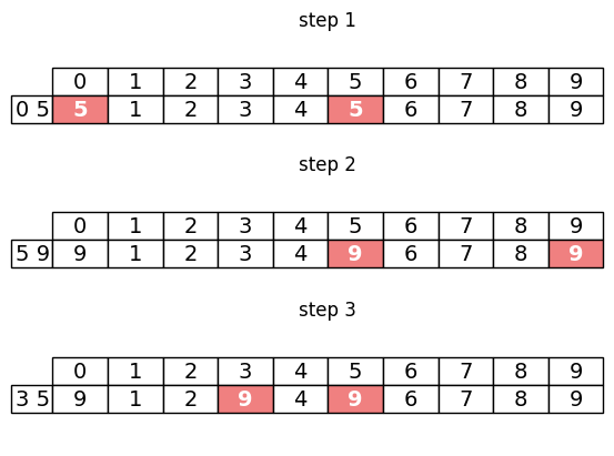
We can see that now, the representative of the 10th item is 8, which is the representative of q (which was 8), meaning the 9th and the 10th item are now merged into the same component. Notice that the 1st items representative has also been set to 8, as the 1st item was in a set with the 10th element, and so it must now also be connected to the 9th item. A graphical representation of this process is shown below. The indices being updated in each step are highlighted in pink.
import matplotlib.pyplot as plt
import numpy as np

columns = [str(i) for i in range(10)]
inp = [(0, 5), (5, 9), (3, 5)]
uf = UnionFind(10)
step = 1
fig, axs = plt.subplots(3, 1)
for ax, (p, q) in zip(axs.flat, inp):
    ax.axis('off')
    uf._union(p, q)
    table = ax.table(cellText=[uf.parents], colLabels=columns, rowLabels=[f"{p} {q}"], loc='center', cellLoc='center')
    table.auto_set_font_size(False)
    table.set_fontsize(14)
    table.scale(1, 1.5)
    for i in (p, q):
        # Cell (row_index, col_index)
        table[(1, i)].set_facecolor('lightcoral')
        table[(1, i)].set_text_props(color='white', weight='bold')
    ax.set(title=f'step {step}')
    step += 1
The algorithm can be run on a complete dataset by calling the class like so.
inp = [(0, 1), (1, 2), (2, 3)]
uf = UnionFind(10)
uf(inp) # loops through all input tuples and updates the parent array
Now that the algorithm has completed we can use the .find method to identify the connected component that each pair reside in. We can use just the first item from each pair, as we know that each pair will have been merged into the same connected component.
print(
    f"{(0, 1)} is in component {uf.find(0)}",
    f"{(1, 2)} is in component {uf.find(0)}",
    f"{(2, 3)} is in component {uf.find(0)}",
    sep='\n'
)
(0, 1) is in component 3
(1, 2) is in component 3
(2, 3) is in component 3
I selected the pair IDs in this example to be mimic the scenario we started this article with, namely that we have 3 complexes which each share a subunit with one other complex. reassuringly, the output tells us that all 3 pairs are in the same component.
Generating splits
Hopefully after that explanation you are comfortable with how UF works. Lets try to apply it to the output from CD-Hit. We parsed the output from the clustering into a list of lists of tuples, with (PDB ID, chain ID, cluster ID). UF requires tuples of IDs however, so we are going to have to mash our data into shape. We need to:
- Group the tuples by their complex
- Turn them into 2-tuples of cluster IDs to feed to UF
Grouping is fairly straightforward. We can use pythons itertools module groupby function. The snippet below creates a dictionary mapping each PDB ID to the cluster IDs of the subunits making up the antigen complex.
from itertools import groupby

max_cluster_id = 0
by_pdbid = {}
for pdbid, g in groupby(sorted(clusters), key=lambda o: o[0]):
    by_pdbid[pdbid] = []
    for subunit in g:
        path, chain, cluster_id = subunit
        if cluster_id > max_cluster_id:
            max_cluster_id = cluster_id
        by_pdbid[pdbid].append(cluster_id)
We are only interested in the complexes that have multiple subunits, so we will collect those.
multi_subunit = {k: v for k, v in by_pdbid.items() if len(v) > 1}
Some complexes have more than two subunits, so we will have to turn those into 2-tuples if we are going to feed them to the UF algorithm. The simplest way to do this is to create pairs from the first subunit with each other subunit.
multi_subunit['5c3l']
[958, 992, 999]
def make_pairs(complex_ids):
    return [(complex_ids[0], complex_ids[i]) for i in range(1, len(complex_ids))]
make_pairs(multi_subunit['5c3l'])
[(958, 992), (958, 999)]
Now we have all the pieces we need to actually run to algorithm. Lets go ahead and do that.
from itertools import chain
pairs = list(chain.from_iterable(map(make_pairs, multi_subunit.values())))
pairs[:5]
[(1034, 1025), (583, 674), (993, 1198), (412, 343), (724, 724)]
uf = UnionFind(max_cluster_id + 1)
uf(pairs)
If we check the number of connected components, we can see that it is less than the number of clusters, meaning several complexes have been merged as due to sharing subunits (or subunits that have a higher identity threshold than the one we initially set in the clustering).
print(f"we started with {max_cluster_id} clusters and ended with {uf.count} connected components")
we started with 1218 clusters and ended with 1033 connected components
Lets now go through the complexes and assign them their componet ID.
components = {pdbid: uf.find(subunits[0]) for pdbid, subunits in by_pdbid.items()}
Lets look for a cluster than has had its ID changed by the UF algorithm.
for pdbid in by_pdbid:
    if by_pdbid[pdbid][0] != components[pdbid]:
        print(pdbid)
        break
1ahw
by_pdbid['1ahw']
[750]
components['1ahw']
1012
c1012 = [p for p, i in components.items() if i == 1012 ]; c1012
['1ahw', '1jps', '1uj3', '4m7l', '5w06', '7ahu', '9p0x']
{k: v for k, v in by_pdbid.items() if k in c1012}
{'1ahw': [750],
 '1jps': [750],
 '1uj3': [750],
 '4m7l': [750],
 '5w06': [750],
 '7ahu': [682, 1012],
 '9p0x': [750, 1012]}
[c for c in clusters if c[0] == '7ahu']
[('7ahu', 'C', 682), ('7ahu', 'D', 1012)]
Looking at the annotations page in pdb for 9p0x and 5w06, we can see that the subunits in cluster 750 are classified as Fibronectin type III domains, while subunits in cluster 1012 are classified as GLA domains, and cluster 682 from 7ahu is classified as Trypsin-like serine protease. This connected component demonstrates exactly the scenario layed out at the start of the post i.e. we have 3 clusters each connected to another by one subunit (in this case: 750, 682 and 1012). This component could not be split between training and testing sets without at least one cluster being shared between the sets.
Use in modelling
In order the use this output in modelling you would need to ensure the each connected component of complexes was put in either train, test or valid. Below is a demonstration of how you might do this in scikit-learn.
group_df = pd.DataFrame.from_dict(components, columns=['group'], orient='index')
group_df.head()
| group | |
|---|---|
| 1a14 | 342 |
| 1a2y | 976 |
| 1adq | 738 |
| 1afv | 709 |
| 1ahw | 1012 |
data_df = group_df.assign(data=np.random.randn(len(group_df))).drop(columns='group').sample(frac=1) # simulate a dataset with the same complexes
data_df.head()
| data | |
|---|---|
| 9myl | 0.598136 |
| 9jub | -0.229788 |
| 9eit | 0.223744 |
| 7yix | 0.317494 |
| 8hp9 | 0.000187 |
from sklearn.model_selection import GroupKFold
splits = GroupKFold().split(data_df, groups=data_df.join(group_df).group) # Match up the rows from the connected components DataFrame with the data using the index.
If you weren’t using a scikit-learn cross-validator and instead wanted to split the data by hand, probably the most effective way is to sort the components by size and distribute them in the following way.
from collections import defaultdict
total_structures = 0
by_component = defaultdict(list)
for pdbid, component in components.items():
    total_structures += 1
    by_component[component].append(pdbid)
by_size = sorted(by_component.values(), key=len, reverse=True)
train_size = int(total_structures*0.8)
test_size = valid_size = int((total_structures - train_size) * 0.5)
train, valid, test = [], [], []
pdbid_iter = iter(by_size)
while len(train) < train_size:
    train.extend(next(pdbid_iter))

while len(valid) < valid_size:
    valid.extend(next(pdbid_iter))

for pdbids in pdbid_iter:
    test.extend(pdbids)
print(f"Train size: {len(train)}\nValid size: {len(valid)}\nTest size: {len(test)}")
Train size: 5512
Valid size: 689
Test size: 690
You could then write these sets out to a file so that you and your colleagues can consitently use the correct held out validation and test sets for any further training your do.
Summary
In this post I’ve introduced to Union-Find algorithm as a quick way of generating highly distinct training and testing datasets for protein structural data. As discussed at the beginning of the post, having a good validation set to test the generalization ability of your model is essential as you iterate on your solution. Without this, you are essentially flying blind! This algorithm is effective and fast for the scale of the data that exists in the PDB. There may be other ways to do this that I am not aware of, and if you know of one, I would love to hear about it! Feel free to reach out to me and tell me about it.