How to use the Observed Antibody Sequence database

All code for downloading and processing the OAS database can be found here

What is the Observerd Antibody Sequence database?

My previous posts have all been quite theoretical, so with this post I thought I would change things up and write a more practical post. We will be working through how to obtain and analyse the Observed Antibody Sequence (OAS) database. The OAS is a database containing millions of antibody sequences captured using Next Generation Sequencing (NGS) across numerous studies. It represents a valuable resource for researchers and engineers in drug discovery, who can use it to understand how the immune system responds to pharmaceutical interventions and disease states, as well as how antibody function relates to their primary amino acid sequences.

The folks at OPIG have done much of the hard work of collating and annotating the sequences in the database, to the great benefit of the community. However, as with any large software project, it has some idiosyncrasies which can be tricky to manage if you are unfamiliar with them. Hopefully this post will provide a roadmap for anyone interested in using this database for their research. The OAS is organized into two collections; the larger ‘unpaired’ OAS which contains unpaired VH and VL sequences and the smaller ‘paired’ database which contains paired VH and VL sequences. I will be working with the paired OAS database in this post, as it is a more manageable size. This tutoral assumes that you are working on a linux OS and have access to python. WSL2 is a fantastic option to be able to use Linux if you have a windows machine.

Fetching and cleaning the database

We will be converting the database to a collection of .parquet files, an open source, column-oriented data file format designed for efficient data storage and retrieval. First however, we will download, clean and re-organize the database. I have deposited the code for this section here so check that out if you want to see all the code in one place. If you go to the paired OAS page and search with no parameters, you will be taken to a page with a download link. This will download a shell script called bulk_download.sh that looks something like this.

wget https://opig.stats.ox.ac.uk/webapps/ngsdb/paired/Eccles_2020/csv/SRR10358523_paired.csv.gz
wget https://opig.stats.ox.ac.uk/webapps/ngsdb/paired/Eccles_2020/csv/SRR10358524_paired.csv.gz
wget https://opig.stats.ox.ac.uk/webapps/ngsdb/paired/Eccles_2020/csv/SRR10358525_paired.csv.gz
...

You could run this script as is (after you have changed its permissions with chmod u+x bulk_download.sh). I prefer to do it slightly differently, as this approach doesn’t take advantage of some of the parallel processing tools on typical Unix systems, and there are alot of URLs to process in this file. What you can do is delete the ‘wget ‘ from the beginning of every line. Then we can use the xargs command to process them in parallel.

export OAS_DOWNLOAD_DIR="${HOME}/Downloads/oas_paired"
xargs -P "$(nproc)" -a oas_paired_urls.txt -I{} bash -c 'curl -sSL -o "$0/$(basename "$1")" "$1"' "$OAS_DOWNLOAD_DIR" {}

The above snippet should result in a set of gzipped csv files being deposited into a “Downloads/oas_paired” subdirectory in you home directory.

$ ls $OAS_DOWNLOAD_DIR | head
1279049_1_Paired_All.csv.gz
1279050_1_Paired_All.csv.gz
...

We can peek inside one of them using the handy zcat utility available on most unix systems, which allows us to read compressed files. If we look at just the first line of one of the files, we can see that there is a json like header line in there with some metadata about the file.

$ zcat ~/Downloads/oas_paired/1279049_1_Paired_All.csv.gz | sed -n 1p
"{""Run"": 1279049, ""Link"": ""https://doi.org/10.1038/s41586-022-05371-z"", ""Author"": ""Jaffe et al., 2022"", ""Species"": ""human"", ""Age"": 35, ""BSource"": ""PBMC"", ""BType"": ""Naive-B-Cells"", ""Vaccine"": ""None"", ""Disease"": ""SARS-COV-2"", ""Subject"": ""Donor-2"", ""Longitudinal"": ""no"", ""Unique sequences"": 8954, ""Isotype"": ""All"", ""Chain"": ""Paired""}"

We will be doing some further processing of this data using python a bit further down the line. Python has a really nice built-in json parser, however if we check this json using a jq (a json parsing cli tool), we see that it is not actually valid json.

$ zcat ~/Downloads/oas_paired/1279049_1_Paired_All.csv.gz | sed -n 1p | jq
"{"
"Run"
": 1279049, "
"Link"
": "
"https://doi.org/10.1038/s41586-022-05371-z"
", "
"Author"
": "
...

Its pretty clear that the culprit is the extra “ around every string, and before and after the json object. We can use sed to surgically remove them to make our lives easier downstream. We will collect all these headers into a new json object mapping filenames to metadata which we can use later. I created a little script which does just that.

extract-json-headers
---
#!/usr/bin/env bash

OAS_DOWNLOAD_DIR="$HOME/Downloads/oas_paired/"
cd "$OAS_DOWNLOAD_DIR"

extract_json() {
  file="$1"
  json=$(zcat "$file" | head -n1 | sed -e 's/""/"/g;s/^.//;s/.$//' | jq -c . 2>/dev/null)
  if [ -n "$json" ]; then
    echo "{\"${file##*/}\": $json}"
  fi
}

export -f extract_json

find . -name '*.csv.gz' -print0 | xargs -0 -n1 -P8 bash -c 'extract_json "$0"' | jq -s 'add'
---

$ ./extract-json-headers > metadata.json

Now that we have extracted and cleaned the metadata from the files, we can process the files themselves. The processing code requires the polars python dataframe library, so if you havn’t already, create a virtual environment and install polars. The main script that does the processing is called csv2parquet.py and can be found here. In order to run it though we need to some further preprocessing.

It turns out that not all the csv files in the paired OAS repository have the same set of headers. A subset of the files are missing several headers. If we extract the headers from all the files and count their fields, we see that most have 198 headers, while some have only 180.

$ ls ~/Downloads/oas_paired/* | xargs -P $(nproc) -I{} sh -c 'zcat {} | sed -n 2p' _ {} > headers.txt
$ awk -F',' '{ print NF }' headers.txt | sort | uniq
180
198

We can drill down a bit more in a python shell. If we look at the headers that are missing from the files that only have 180 fields, we can see that both the heavy and light framework 4 amino acid sequences are missing in these files. I suspected this is because only partial sequencing was carried out in these runs, and the framework 4 sequences weren’t captured. In any case, we need all our parquet files to have the exact same number or columns, and the amino acid sequences of the framework 4 regions are likely to be important to our downstream analysis. As there are only 17 of these files, we will remove these files during our processing.

>>> from pathlib import Path
>>> lines = [line.split(',') for line in Path('headers.txt').read_text().splitlines()]
>>> shortheaders = [line for line in lines if len(line) == 180]
>>> longheaders = [line for line in lines if len(line) != 180]
>>> set(longheaders[0]) - set(shortheaders[0]) # computes set difference
{'fwr4_light', 'Redundancy_heavy', 'Redundancy_light', 'Isotype_light', 'fwr4_aa_light', 'v_frameshift_heavy', 'fwr4_heavy', 'fwr4_start_heavy', 'complete_vdj_heavy', 'complete_vdj_light', 'fwr4_end_heavy', 'c_region_light', 'c_region_heavy', 'fwr4_start_light', 'fwr4_end_light', 'Isotype_heavy', 'fwr4_aa_heavy', 'v_frameshift_light'}
>>> len(shortheaders)
17

Our next step will be to actually process the compressed csv files and convert them to parquet. All data stored on the OAS conforms to the Adaptive Immune Receptor Repertoire standards. These are a set of community agreed rules that specify what data should be included in a sequencing data submission, how that data should be named, and what their types should be. I have used this to define a type mapping in csv2parquet.py, which specifies how polars should type each incoming column. Without this, polars would try to infer the type of each of the columns in the csv files by looking at a subset of the rows. As well as being slow, this is error prone, so specifying them up front is a good idea. To be safe, we can ensure that we are only parsing fields that exist in the csv files using the snippet below. The ‘commonheaders’ file will be passed as input to the csv2parquet.py file.

$ awk -F',' 'NF == 198 { print $0 }' headers.txt | tr ',' '\n' | sort | uniq -c | awk '$1 == 563 { print $2 }' > commonheaders

With all this done, we are ready to run the primary processing pipeline. We supply it with the directory containing the compressed csv files, a directory to write the outgoing parquet files (which I am just calling parquets), and the ‘commonheaders’ file we just created to ensure we are processing the correct fields.

./csv2parquet.py $OAS_DOWNLOAD_DIR parquets commonheaders
$ ./csv2parquet.py $OAS_DOWNLOAD_DIR parquets commonheaders
2025-06-15 09:50:02,997 - INFO - Processed 1287202_1_Paired_All.csv.gz successfully.
2025-06-15 09:50:03,881 - INFO - Processed 1287195_1_Paired_All.csv.gz successfully.
2025-06-15 09:50:04,301 - INFO - Processed Human_colon_16S8157815_S27_1_Paired_All.csv.gz successfully.
2025-06-15 09:50:04,619 - INFO - Processed SRR27484729_1_Paired_All.csv.gz successfully.
...

You should get a stream of logs telling you which files have been successfully processed. All in all the script took just under 4 minutes to run on my machine, but your mileage may vary. If we peek into the parquets directory we will see lots of shiny new parquet files. One advantage of parquet files becomes obvious if we check the size of the input and output directories. The parquets together take up roughly half the disk space that the compressed csvs did. Granted we left a handful of csvs out due to the column truncation issue, but there were only a handful and are unlikely to account for the differences we see here.

$ du -sh parquets
2.0G    parquets
...
$ du -sh $OAS_DOWNLOAD_DIR
5.2G    ~/Downloads/oas_paired

Querying the data

Variable domain germline preferences

Now that we have obtained and scrubbed the database. We can continue with the fun part - asking questions of our data. A really interesting piece of work by Clarissa A. Seidler and colleagues at the Liedl lab looked into intrinsic pairing preferences between heavy and light variable domains using the paired OAS database. This question has practical significance in antibody engineering scenarios. We often need to choose a light chain to pair with a heavy chain, for example when we humanize mouse antibodies, or potentially for an optimization campaign. In this context, knowing that some light chains represent poor partners for a given heavy chain is important. This work is also an excellant example of the kinds of questions that can now be answered with clean, diverse and large scale antibody repertoire data. Lets see if with can emulate some components of their analysis and extend it with some of our own.

import matplotlib.pyplot as plt
import polars as pl
from scipy.stats import chi2, norm
import numpy as np
import seaborn as sns
import seaborn.objects as so
from scipy.stats import norm

I carried out this analysis in a Jupyter Notebook. The first thing we can do is load the data and check how many sequences we have. The nice thing about polars, is that we can pass it a glob string that expands to a collection of parquet files, and it will allow you to write queries over them as if they were a single table!

The output tells us there are 2965738 sequences. This is slightly lower than the 3,087,576 that is the result of a blank search on the OAS website (at the time of writing), probably due to those trucated header files we dropped, but this should be more than enough for our purposes.

lf = pl.scan_parquet('parquets/*.parquet')
print(f"Total sequences: {lf.select(pl.len()).collect().item()}")

Total sequences: 2965738

VH - VL Pairing Preferences

A core component of Seidlers work was to compare the expected distribution of light V genes with that that which was observed and test the significance of the deviation from expectation using the \(\chi^2\) test.

\[\chi^2=\sum \frac{\left(O_i-E_i\right)^2}{E_i}\]

# Count pairing frequencies of heavy and light V genes
counts = lf.group_by(pl.col("v_call_light", "v_call_heavy")).agg(pl.len()).collect()

# Create a contingency table
dfpandas = counts.to_pandas()
contab = dfpandas.pivot_table(index='v_call_heavy', columns='v_call_light', values='len').fillna(0)
contab = contab.loc[contab.sum(1).gt(100),contab.sum(0).gt(100)]

total_seqs = contab.values.sum()
hc_totals = contab.sum(axis=1).values
lc_totals = contab.sum(axis=0).values
expected = np.outer(hc_totals, lc_totals) / total_seqs

chisq_stat = ((contab - expected) ** 2 / expected).values.sum()
degfreedom = (contab.shape[0] - 1) * (contab.shape[1] - 1)
pval = 1 - chi2.cdf(chisq_stat, degfreedom)
print(f"P-value: {pval}")

P-value: 0.0

The p-value we get out is 0.0, which tells us there is effectively 0 chance that the difference we are seeing between our observed and expected frequency distributions of light variable genes could have been observed were there no dependance on the heavy variable gene, which is what they showed in the paper. If we were looking at a single study only, then you might suspect that the pairing preferences were an artifact of the sampling process. For example, perhaps a particular heavy light germline pair respond particularly well to the flu vaccine components, which many of the study participants had just received. However, according to Seidlers et al, This preference showed up across studies with varied populations, so its probably safe to say this is a real phenomena we are observing. The authors speculate that these preferences may be driven by charge interactions, although the full determinants seem to remain somewhat elusive.

VL HCDR3 Loop Length Interaction

Another relationship that could be interesting to look at is that between the light germline family and the length of the heavy CDR3. i.e. are there some light germline families that support longer heavy CDR3s? Lets first compute the lengths and then check that they make sense.

lf = lf.with_columns(pl.col("cdr3_aa_heavy").str.len_chars().alias('cdr3_aa_heavy_len'))

longest_hcdr3s = lf.sort(by='cdr3_aa_heavy_len', descending=True).select('cdr3_aa_heavy_len').limit(100).collect()

print([l for l, in longest_hcdr3s.rows()])

[77, 58, 53, 52, 52, 50, 49, 49, 48, 47, 46, 46, 44, 44, 43, 43, 43, 42, 42, 42, 42, 42, 42, 42, 41, 41, 41, 41, 41, 41, 41, 41, 41, 40, 40, 40, 40, 40, 40, 40, 40, 40, 40, 40, 40, 40, 40, 40, 40, 40, 40, 40, 39, 39, 39, 39, 39, 39, 39, 39, 39, 39, 39, 39, 39, 39, 39, 39, 39, 39, 39, 39, 39, 39, 39, 39, 39, 39, 38, 38, 38, 38, 38, 38, 38, 38, 38, 38, 38, 38, 38, 38, 38, 38, 38, 38, 38, 38, 38, 38]

Looking at the top 100 amino acid lengths, some of them seem very long, possibly representing an problem with the data. To be save we can just filter out these longer CDRs.

lf = lf.with_columns(pl.col("cdr3_aa_heavy").str.len_chars().alias('cdr3_aa_heavy_len')).filter(pl.col('cdr3_aa_heavy_len') < 40)

fig, ax = plt.subplots()
ax.ecdf(lf.select('cdr3_aa_heavy_len').collect().to_numpy().squeeze());

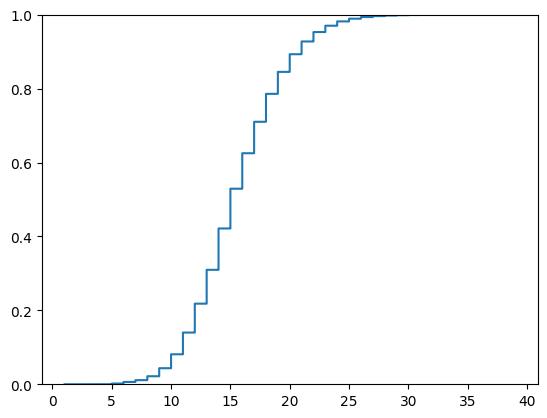
A cumulative distribution plot shows that the large bulk of the sequences are shorter than 30 amino acids in length, so a cut off of 40 seems safe.

We can plot the counts for the top 25 most frequence light chain genes to get a feel for their distribution.

v_call_counts = lf.group_by('v_call_light').agg(pl.len().alias('count')).select('v_call_light', 'count').collect()

df = (
    v_call_counts
        .sort(by='count', descending=True)
        .top_k(25, by='count')
        .to_pandas()
)
ax = df.plot.barh(x='v_call_light', y='count')
ax.tick_params(labelsize=7)

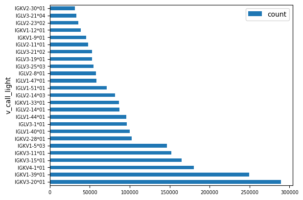
Clearly some gene families are much more frequent than others, with IGKV3-20*01 coming up the most.

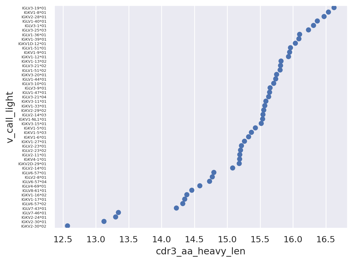
Lets look at the mean CDR3 lengths broken down by light gene family for the top 50 most frequently occuring families.

top50_light_gls = lf.group_by('v_call_light').agg(pl.len()).top_k(50, by='len').select('v_call_light')
lf = lf.join(top50_light_gls, on='v_call_light', how='semi')
lf = (lf
    .with_columns(
        pl.col('cdr3_aa_heavy_len').median().over('v_call_light').alias('median_hcdr3_len'),
        pl.col('cdr3_aa_heavy_len').mean().over('v_call_light').alias('mean_hcdr3_len')
    )
    .sort(by='mean_hcdr3_len', descending=True)
)
df = lf.select('v_call_light', 'cdr3_aa_heavy_len').collect()

It looks like the average heavy CDR3 length is ~16

df['cdr3_aa_heavy_len'].mean()

15.581879397897739

The graph below clearly shows that there are differences in average heavy CDR3 length across different light germlines. It appears that IGLV3-19*01 has the longest heavy CDR3s on average, while the IGKV2-30 family *01 and *02 alleles have the lowest. This could be because these light chains are intrinsicly less able to support longer heavy CDR3s, possibly for structural reasons, however it could also be because these light chains preferentially pair with heavy chains that tend to display shorter CDR3s regardless of light chain V gene partner. In other words it is not clear which way the arrows of causality point.

p = so.Plot(df, x='cdr3_aa_heavy_len', y='v_call_light').add(so.Dot(), so.Agg('mean'))
p = p.layout(size=(5, 10)).theme({'ytick.labelsize':8})
p

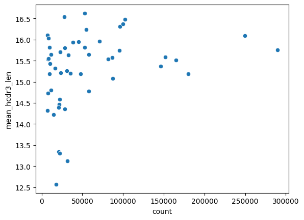
An additional possibility is that these light germline gene families have a small sample size and the effect we are seeing is more a product of noise than any real biological effect. If we plot the mean heavy CDR3 length against sample size it does look like there are fewer light germline families paired with shorter heavy CDR3s at the higher sample sizes.

df = lf.group_by('v_call_light').agg(pl.len().alias('count'), pl.col('mean_hcdr3_len').first()).collect()
sns.scatterplot(df, x='count', y='mean_hcdr3_len');

lf.filter(pl.col('v_call_light').is_in(['IGKV2-30*01', 'IGKV2-30*02'])).select(pl.len()).collect().item()

49540

There are ~50000 sequences from the two light germline families with the shortest heavy CDR3s. This seems like a fairly large sample size; large enough that we are unlikely to see average lengths this short by chance. Lets check this though.

sns.histplot(lf.select('cdr3_aa_heavy_len').collect(), binwidth=1)

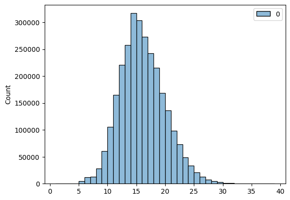
The distribution of heavy CDR3 lengths is roughly gaussian. We can estimate the population parameters from the entire dataset and use these to do a one-sided Z test.

cdr3_aa_heavy_lens = lf.select('cdr3_aa_heavy_len').collect()
mu_hat = cdr3_aa_heavy_lens.mean().item()
sigma_hat = cdr3_aa_heavy_lens.std().item()
igkv2_30 = lf.filter(pl.col('v_call_light').eq('IGKV2-30*02')).select('cdr3_aa_heavy_len').collect()
y_bar = igkv2_30.mean().item()
m = igkv2_30.height

The difference between the means of our larger sample and the IGKV2-30*02 gene is large enough that it is almost certainly not due to chance.

f"P-Value: {norm.cdf((y_bar - mu_hat) / (sigma_hat / math.sqrt(m))).item():.10f}"

'P-Value: 0.0000000000'

Although the differences are not due to chance, they could be lower due to their preferential pairing with heavy chains that carry shorter CDR3s. Lets look at this. Looking at the differences between observed and expected pairing counts for IGKV2-30*02 and heavy germline V genes. It looks like IGKV2-30*02 pairs with IGHV3-9*02 much more frequently than expected.

((contab - expected) / expected).filter(like='IGKV2-30*02').sort_values(by='IGKV2-30*02', ascending=False)

v_call_light	IGKV2-30*02
v_call_heavy
IGHV3-9*02	43.801180
IGHV3-7*05	6.133745
IGHV3-30*10	5.560173
IGHV3-7*01	4.666647
IGHV3-7*02	4.100613
...	...
IGHV4-31*04	-1.000000
IGHV4-30-2*06	-1.000000
IGHV4-59*03	-1.000000
IGHV4-61*10	-1.000000
IGHV7-4-1*01	-1.000000

187 rows × 1 columns

The average heavy CDR3 length for IGHV3-9*02 is actually far lower than the average across the entire dataset.

lf.filter(pl.col('v_call_heavy').eq('IGHV3-9*02')).select(pl.mean('cdr3_aa_heavy_len')).collect().item()

12.491721854304636

g = sns.histplot(lf.select('cdr3_aa_heavy_len').collect(), binwidth=1)
g.axvline(12.5, c='red')
plt.show()

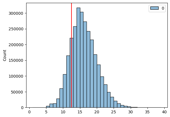
The short heavy CDR3 length of the preferential heavy V gene partner for IGKV2-30*02 likely explains the short heavy CDR3s we observed for this light V gene family. If the light chain was having an independant effect on the heavy chain CDR3 length distribution then we would likely only see a downward shift in CDR3 lengths when conditioning on the light V gene, however we see this shift in its absence, suggesting the relationship is more likely correlative than causal. It is possible that if we conditioned on the light chain V gene we would get a significant downward shift in the average CDR3 length, however the effect size of this shift would likely be diminutive and unlikely to have real world practical applications.

Summary

This was a very quick and informal analysis, just to give you a sense of the power of this dataset as well as some guidance on tools and techniques to use for analysing it. While the light V germline pairing choice effects on heavy CDR3 lengths may seem inconsequential, a better understanding of these nuanced features of antibody biology in the aggregate will help antibody engineers to make the next generation of improved therapeutics and tools. Therefore I hope to see some of you playing around with these datasets and publishing your findings!